

Next: Summary of the
Up: Wind Profiling Method
Previous: Estimating Mean Wind
Return to the Publications.
Return to the Index.
The most effective way to calculate time-averaged wind estimates is
to average the cross correlation functions over a time period.
This provides a less noisy correlation function to the wind calculation,
since random correlations vanish in the averaging process.
Even a weak aerosol correlation peak
dominates the cross correlation function after an appropriate averaging time.
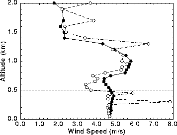
Figure 27 compares the results of two averaging methods.
The first method averages subsequent correlation functions to produce
a consistent wind profile.
The second method averages the wind estimates calculated from
shorter time-average cross correlation functions.
Some estimates from the second method
have large fluctuations between adjacent points due to
spurious results which were averaged with more accurate results.
All results presented in this study are generated by averaging correlation
functions.

Figure 27:
Wind profiles after different averaging methods on August 9, 1989,
from 10:30 to 10:45 CDT.
The solid line with solid circles is a wind profile
calculated from the average of five subsequent cross correlation functions.
The dashed line with open circles is a wind profile
calculated by averaging five wind profiles estimated from
individual subsequent cross correlation functions.
The vertical dashed line at 500 m marks
the convective boundary layer mean depth.
Antti Piironen
Tue Mar 26 20:53:05 CST 1996


